At Wealthfront, we use A/B tests to make our services more effective, informative, and convenient. Each A/B test consists of two or more variants of a feature or design, which we expose to visitors at random until we have have enough data to infer which is better. In a previous post, we explained why we use Bayesian inference for evaluating A/B tests. Today I will share a technique we use to avoid inference errors on A/B tests with many variants: a concept called shrinkage. We’ll start with a hypothetical use case that everyone can relate to: bananas.
Running tests at the online banana stand
Let’s say you work for a popular online banana stand, and I ask you what proportion of banana stand visitors purchase a banana. Without any data, it would be reasonable to assume that the proportion $theta_text{control}$ is a value somewhere between 0% and 100% with equal probability. While the proportion is a fixed value, this probability distribution captures our uncertainties in its true value. The essence of Bayesian statistics is updating this distribution as we get more data.
Now what if you know the proportion of banana stand visitors who buy a banana, and I ask you what the proportion will be if you change your website’s buttons from green to pink? You have no data about this scenario, so you’ll have to guess again, but it is likely that this new proportion, $theta_text{pink}$, is close to the original proportion, $theta_text{control}$. Shrinkage is the technique we use to incorporate this intuition into our Bayesian model. As we collect data, using shrinkage helps us carefully discern whether visitors prefer the pink buttons to the green ones. Before we explain shrinkage in detail, let’s cover how Bayesian models work.
Bayesian models
As mentioned above, a simple assumption is that $theta_text{control}$ is uniformly distributed between 0 and 1. Mathematically speaking, that means the probability density $P(theta_text{control})$ is constant between $theta_text{control} = 0$ and $theta_text{control} = 1$; $P(theta_text{control}) = 1$. We can easily update this distribution as we collect more data $D$. If I observe a random visitor and find out that they buy a banana, I have a data point $y_1=1$, and Bayes rule states that the probability of $theta_text{control}$ given this information $D = {y_1 = 1}$ is [P(theta_text{control}|D) = frac{P(theta_text{control})P(D|theta_text{control})}{P(D)} qquad [1]] We already decided that $P(theta_text{control}) = 1$. By definition, $theta_text{control}$ is the proportion of visitors that purchase bananas, so the probability $P(D|theta_text{control})$ of observing that this person bought a banana, given $theta_text{control}$, is just $theta_text{control}$. Plugging in these two facts to equation [1] gives us that [P(theta_text{control}|D) = frac{theta_text{control}}{P(D)} qquad [2]] The only thing we don’t know yet is $P(D)$, which we can calculate by enforcing that the total probability is 1: [int_0^1P(theta_text{control}|D)dtheta_text{control} = 1] Using equation [2], [int_0^1frac{theta_text{control}}{P(D)}dtheta_text{control} = 1] Since $int_0^1theta_text{control}dtheta_text{control} = 0.5$ and $P(D)$ is independent of $theta_text{control}$, this becomes [frac{0.5}{P(D)} = 1] This implies that $P(D) = 0.5$, so the probability $P(theta_text{control}|D) = 2theta_text{control}$.
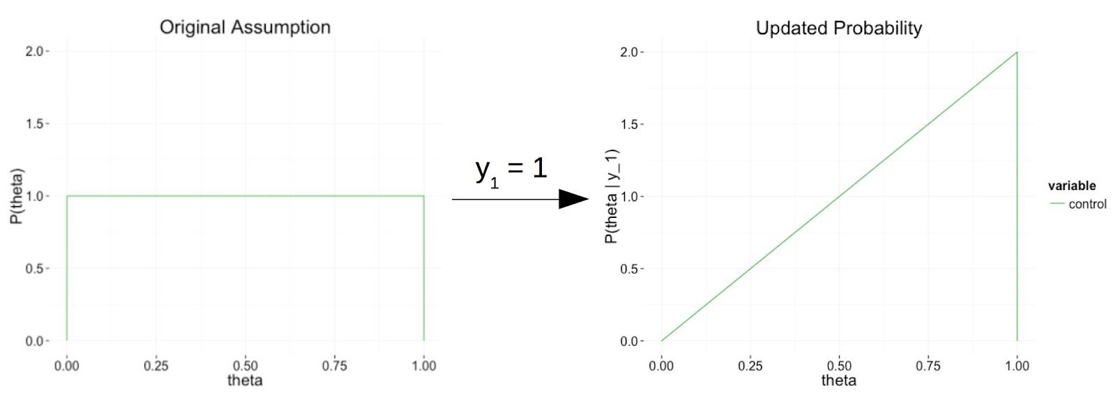
The intuition behind this result is that, since we observed someone buy a banana, the proportion of visitors who buy bananas must be greater than 0. Based on this evidence, it is also more likely to be high than low, but we will update that claim as we collect more data.
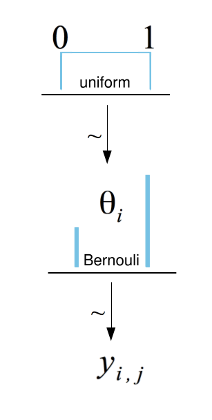
In this way, we can use our observations $D$ to update our estimate of how likely each possible value of $theta_text{control}$ is. The model can be summarized by this diagram at right. This diagram can be read from bottom to top to say that our observations $y_j$ are randomly 0 or 1 with some likelihood $theta_text{control}$, and that we assume $theta_text{control}$ could be uniformly anywhere between 0 and 1, which we will update as we observe data. The top distribution shown is our initial assumption, and each variable is assumed to be drawn from the distribution(s) above it. If we collect enough data $D = {y_1 = 1, y_2 = 0, y_3 = 0, ldots}$, we may end up with a probability distribution like this:
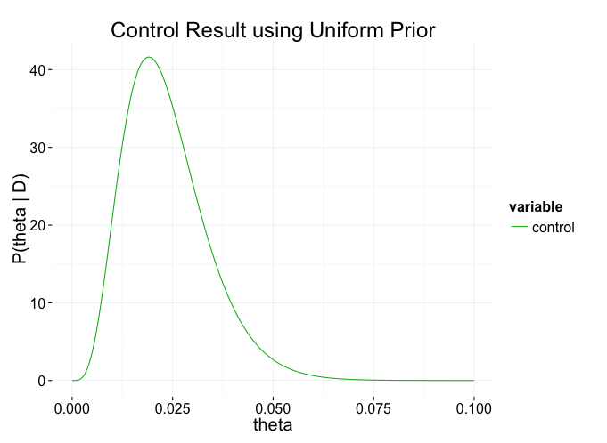
The more data we collect, the more precisely we can estimate $theta_text{control}$.
Multiple comparisons
Suppose we test three different button color changes (plus control) and collect this data:
| Variant | Purchases | Visitors |
| control | 4 | 210 |
| pink | 1 | 200 |
| blue | 4 | 190 |
| yellow | 6 | 220 |
The model we just described would give the following probability distributions:

According to this model, there is more than a 95% chance that yellow buttons are more attractive than pink buttons. But we are comparing 4 proportions, meaning that we are doing 6 pairwise comparisons, so we actually have much more than a 5% chance of making an error. As we compare more proportions simultaneously, the risk of making a random error dramatically increases. The frequentist method to deal with this is to require higher confidence for each comparison. This is called the Bonferroni correction. In our example, since we are doing 6 comparisons, we should require $1 – 0.05/6 = 99.2%$ confidence in each of our comparisons. This is a high bar, and it means that we need to collect substantially more data.
There’s no getting around the fact that we need more data, but fortunately we (usually) don’t have to worry about multiple comparisons with Bayesian statistics. Rather than use the Bonferroni correction, we can simply use a different model with shrinkage. And rather than resolve to collect a huge number of data points, we can end the experiment whenever its result becomes significant, which happens faster if the difference between variants is more pronounced.
Shrinkage
Previously we started with the assumption that any proportion $theta_i$ is equally likely before we collected any data. Since it is related to the other $theta_i$ proportions, though, a better assumption is that the proportions $theta_text{control}$, $theta_text{pink}$, $theta_text{blue}$, $theta_text{yellow}$ all share a common distribution. This is a compromise between the frequentist null hypothesis that all $theta_i$ are equal and the original Bayesian model, which treats all $theta_i$ as totally unrelated quantities.
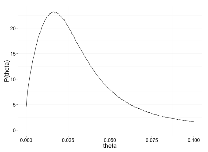
For this fictional example, we can see that the $theta_i$ are clustered around roughly 0.02 (is it extremely unlikely that four uniformly random proportions would all be in such a small interval). To quantify this, we make another Bayesian model for the distribution of the means, and update it as we collect more data. Intuitively, since the proportions we want to measure are related, they are probably more similar than we observe. In the extreme case, if all $theta_i$ truly are exactly equal, any deviations in the data would be random effects.
In the model for the parameter means, we assume all $theta_i$ are drawn from a beta distribution with mean $omega$ and spread $k$. In this way, the closer together the sample means, the tighter our predicted distribution for them becomes. For our observed means in this example, the estimated distribution over $theta_i$ parameters looks roughly like:

We use this in place of the uniform prior distribution we had before. By coupling our original model with this new distribution for each $theta_i$, we create the hierarchical Bayesian model at right.
This model assumes that each visitor observing variant $i$ has a chance $theta_i$ to buy a banana. Each proportion comes from a common distribution of banana purchase rates, and we have prior assumptions about the mean $omega$ and spread $k$ of that distribution. These distributions all work together to give us more accurate estimates of each $theta_i$.
This model “shrinks” our proportions toward their common mean, so that until we have enough data to prove otherwise, we make conservative estimates about the parameter differences. Here is the plot of our new predicted distributions for each color:

In our banana stand example, our estimate for how much greater $theta_text{yellow}$ is than $theta_text{pink}$ drops from 261% to 113%, and our confidence that the difference is positive drops from 95% to 90%.
More practical data
I generated random data to see how well each inference method worked. The random data comes from the following hypothetical scenario: suppose we have 4 variants with exact banana purchase proportions 2%, 2.2%, 2.4%, and 2.6%. We watch 300 visitors for each variant, then run our inference methods to estimate the distribution of each proportion.
I ran this simulation 1000 times and counted
- the number of trials where any type S errors (where $theta_1$ is predicted to be greater than $theta_2$ when actually $theta_2 > theta_1$) occurred
- the average mean squared error of both models:
| Model | Trials with S errors | Mean squared error |
| with shrinkage | $24$ | $1.9times10^{-3}$ |
| without shrinkage | $42$ | $2.1times10^{-3}$ |
With high confidence (using whichever frequentist or Bayesian inference method you want), we can say that including shrinkage prevents us from making some spurious type S errors and gives us more accurate results overall in this scenario.
It may seem counterintuitive that shrinking the parameters together gives a more accurate result, but it turns out that under a normal model for at least three parameters, there is a factor by which you can shrink the observed means in any direction and obtain a more accurate result on average; this factor is called the James-Stein estimator.
Summary
You may still have doubts as to whether shrinkage is truly the best way to avoid inference errors. The truth is that any inference method makes a tradeoff between power (chance of discerning which quantity is actually greater) and low error rates. Shrinkage is a technique that allows us to trade power for low error rates. Its advantage is that it is perfectly suited to our application: the measurement of similar quantities with multiple comparisons. It intelligently makes more conservative estimates in accordance with this similarity. At Wealthfront, it helps us sleep at night to know that our experiments are resolved with both the precise, unbiased automation of a computer while incorporating sane intuition of a human.