
At Wealthfront, a core pillar of our business model is addressing our clients’ needs proactively, efficiently, and with minimal unnecessary toil. As our client base grows, and as we ship an ever broader suite of products and features, the breadth of issues our support and operations staff have to address grows as well. Our preference has always been to scale with automation and targeted investment in systems that address these issues before they ever reach our team. So how do we sort through an ever growing list of client needs and pick out the most impactful initiatives we can pursue to address them? The first step is visibility. This post will explore how we achieve that visibility into one of our highest volume support channels, phone calls.
Our Dataset
For years, Wealthfront has staffed our support line with real people. We have no exhaustive phone tree to listen and tap through. We don’t have an extensive system recording and analyzing each call. The phone rings and one of our Product Specialists picks up the line. In fact, the only hard data we retain about each call is the time, incoming number, and duration. Additionally, our representative may take notes on the subject of the call and any actions taken on the client’s behalf for future reference. While we think this process creates the best client experience, it is not optimized for our goal of visibility.
Here are a few examples of notes taken from calls with a client:
“Called to ask for 401k check rollover info”
“Called – Inquired about Roth conversion process. Explained funds would first get invested in Traditional IRA. After funds clear, he can convert Trad IRA to Roth IRA.”
“Called asking how to wire to escrow for the purchase of a home. I let him know he can submit a wire to escrow for the purchase of a home in his name directly from the app or website. I gave him the general timeline and to have purchase agreement and wire doc handy just in case”
As you can see, the notes vary greatly in structure and detail.
Topic Discovery
In order to create visibility, we need a way to analyze those notes at scale. Of course we could review, label, and tabulate call topics by hand. Surely we can do better with automation.
The old way
Topic modeling is not a new art. Traditional NLP (Natural Language Processing) has been working to address this problem for decades. By counting the occurrence of specific words in each note, we can map them to vectors where the dimension is the total number of distinct words in the corpus and the value in each position is the count of that word. That gives us a mathematical structure to group notes by which words co-occur between them. This is an extremely simple model. There are probably many obvious improvements that come to mind even reading the description. We could consider phrases instead of just words, incorporate the order of words in some way, filter out unimportant filler words, merge synonyms into the same count… The list goes on.
Using an LLM
The field of AI research has been hard at work solving these problems generally, and we can jump straight to the end of all our proposed improvements with the modern LLM. In fact, LLMs are so powerful and competent at general language processing tasks that maybe they can solve our problem right out of the box. If we hand each note to a frontier LLM like Sonnet or GPT 5, surely it can tell us the topics covered in that call.
For example, if we send an LLM three notes and ask it to identify the topic of each:
| Note | LLM Output |
|---|---|
| “Called – wanted to know if he could get check. told him to submit online.” | Check delivery inquiry |
| “Asked for stop payment on check, estimated date was yesterday” | Check stop payment request |
| “Client called about APY rate on cash account.” | Interest rate question |
This approach seems to work, but it has several problems. First, we want consistent output topics for analytical use. The labels work in isolation, but there is no guarantee of consistency. Another very similarly worded note about the cash account APY might get labeled “Question about interest rates” instead. To get consistent labels, we need to provide a list of possible labels for the model to choose from along with the note. We don’t have a list of topic labels yet – that’s our whole goal. Second, it is slow and expensive. You have to put every note before an expensive and slow LLM along with an extensive description of the labelling task required of it. Depending on the volume, the time and money may easily be worth the result, but we can do better.
The middle ground
Luckily, there is a happy medium between a bag-of-words that we train ourselves and a giant model suited for any language-based task: embedding models. What is an embedding? Simply put, an embedding is a vector of fixed dimension that densely encodes the meaning of a piece of text. They encode far more than the presence of certain words and phrases in a text. They are also very fast to calculate compared to the output of an LLM. In fact, they are an integral part of the inner workings of LLMs. And they have many uses in their own right. One common use is semantic search, where a simple vector distance calculation can return the documents closest in meaning to your query from a large corpus of documents. To solve our topic discovery problem, we want to do something similar where we detect clusters of documents that are close to each other in the embedding vector space.
Quantify with Embeddings
The first step is to embed each note. Embedding models are actually small enough to host on a machine with a decent GPU, but the quickest way to get off the ground is to use a cloud hosted model. OpenAI’s text-embedding-3-small is a reasonably priced option that should be suitable for this task.
import OpenAI from "openai";

const openai = new OpenAI();

const embedding = await openai.embeddings.create({
  model: "text-embedding-3-small",
  input: call_note,
  encoding_format: "float",
});
Code language: Python (python)
After embedding each of our notes, we are left with a set of 1,536 dimension vectors. This is actually far more dimensions than we need and that could muddy the result of the clustering operation. To conceptualize why, note that our embedding model was trained on the full breadth of text available to the researchers at OpenAI. In the universe of text of all possible forms and contents, our entire corpus is already a relatively tight cluster of “notes taken by a representative on a call with a client”. To address this, we use the UMAP operation to compress our data into a lower dimension vector space. You can think of this like flattening out all the dimensions that don’t vary much between vectors in our dataset and preserving the ones that do.
import umap

compressed_embeddings = umap.UMAP(
    n_components=25,
    n_neighbors=30,
    min_dist=0.0,
    metric="cosine",
).fit_transform(embeddings)
Code language: Python (python)
Cluster with HDBSCAN
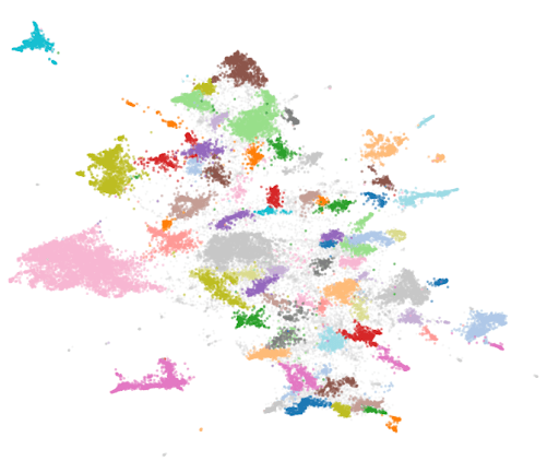
At this point we have transformed each of our notes into a vector of 25 elements. Just as a vector of 3 elements can be interpreted as coordinates in 3-dimensional space, you can think of our vectors as coordinates in 25-dimensional space. Each note’s location in this space is determined by its semantic meaning relative to the other notes. Now we want to run a clustering algorithm to identify groups of notes that are near each other in the vector space, indicating that they have similar meaning. To start with, we are going to use the HDBSCAN algorithm. This is an efficient, unsupervised learning algorithm that can be used to compute a set of flat clusters that each have a minimum size. After choosing some reasonable default parameters and applying it to our data, we are left with 89 distinct clusters.
from sklearn.cluster import HDBSCAN

clusters = HDBSCAN(
    min_cluster_size=100,
    min_samples=15,
    metric="euclidean",
    cluster_selection_method="eom",
).fit_predict(compressed_embeddings)
Code language: Python (python)
To visualize the result, we can use UMAP again to project our data down to just 2 dimensions and plot it. We lose quite a bit of fidelity by eliminating 23 dimensions from our vector space, so the visualization has more aesthetic than analytical value.
Hierarchical Sub-clustering
We’ve made great progress, but there are certainly more than 89 things our clients call in about. Depending on the desired application of the output topics we discover, we may want them to be more specific. We could solve this by going back to our HDBSCAN parameters and tuning them so the data is sliced into many smaller topics. This fulfills our desire of specificity, but we lose visibility into which of these smaller topics actually fall within one of the original larger clusters. If one of the original topic clusters corresponds to part of the product owned by a specific team, we don’t want to have to pore over hundreds of more specific topics and figure out which of them pertain to that product in order to provide useful data to that team. There is no reason we have to limit ourselves to clustering all the data at once, though. We can have our cake and eat it too.
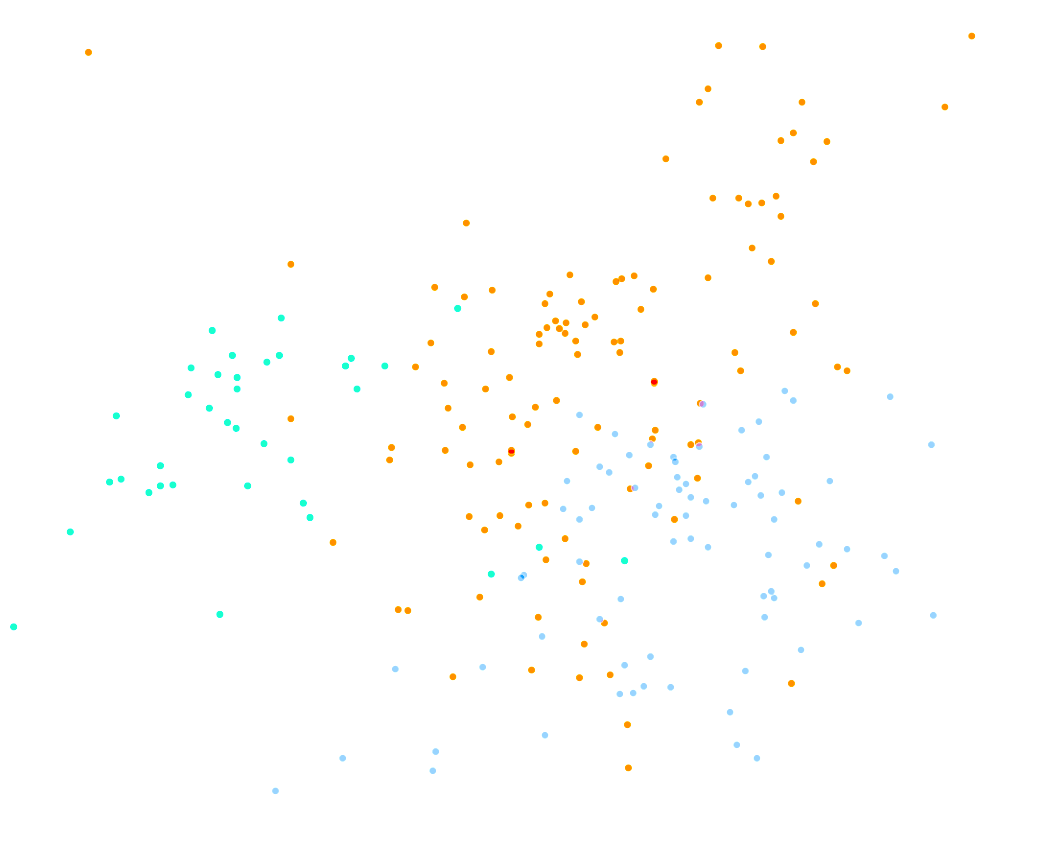
To create a two-tier hierarchy of sub-topics, we can repeat the process of clustering within each of our original large clusters. For each cluster, we take only the notes assigned to that cluster and UMAP them down to even fewer dimensions than the first time. We know they have a lot of semantic similarity with each other, and now we want to tease out the differences. Then we run HDBSCAN again, choosing parameters that allow us to discover smaller distinct clusters than the original pass. We are rewarded with hierarchical topic classification that can be used to explore trends in large umbrella topics, or drill down and look at what exactly clients call in about for a specific part of the product.
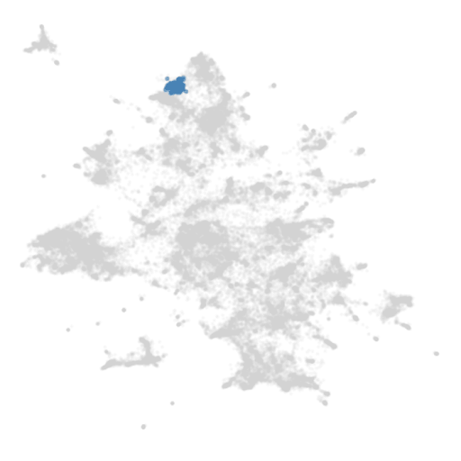
If we again map our data down to 2 dimensions to visualize, we can see how one of the original clusters has been broken down into 3 distinct sub-clusters.
Labelling the Clusters
As useful as our result is so far, you may have noticed something missing. Our clusters are each only described as a subset of our original notes, and can only be referred to by an index assigned to them by the clustering operation. We need a way to create actual topic labels for them. This is a job for the big reasoning LLM we set aside earlier. If we take a sampling of the notes in each cluster, an LLM should be able to read them and identify the common thread in their topics to create a name for the cluster. We need to be careful though. If we bias our selection of sample notes (e.g. by selecting the ones with the earliest timestamps) the LLM might name our cluster too specifically in a way that doesn’t capture the full breadth of topics it encompasses.
Imagine a cluster contains the notes of all calls about tax documents. If we grab the first 10, they might all come from January. That’s when 1099s get released, so most of them might be about 1099s. The LLM would understandably name the cluster “1099 Form Inquiries.” This obscures the fact that the cluster also contains notes from later months about W-9 uploads, tax loss harvesting statements, and foreign tax credits.
Since we already created sub-clusters of our top-level clusters in the last step, we can sample notes from near the centroid of each sub-cluster for unbiased labelling of the parent cluster. This doesn’t work for our smallest tier of clusters, but sampling randomly should get us close. In practice, we actually run three tiers of clustering for even more specific sub-topics at the lowest tier. The third tier does help with sampling notes to name the second tier, but beyond that has limited analytical use because there are too many labels to reason about at a high level.
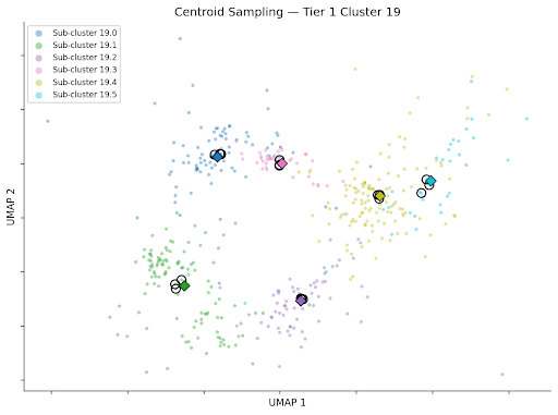
The notes closest to each centroid capture the core theme of their sub-cluster. For example, from two sub-clusters within “Check deposit and account questions”:
Check status & delivery:
“Called – Inquired about check status. Explained that we do not see a check sent because it appears we didn’t receive their check confirmation in time.”
Check deposit guidance:
“Client called in about rollover check — wanted to know if he can mobile deposit. Explained he cannot and will need to mail to us.”
Here is a sample of our final topic hierarchy, showing how broad clusters of topics from our first pass break down into specific sub-topics:
Wires and funding methods
  ├─ Wire transfers & real estate
  ├─ Third-party wires
  ├─ Wire status & processing updates
  └─ ...

Tax Forms & Residency
  ├─ Tax Documents and 1099s
  └─ W9 and Tax Forms

Login and Access Issues
  ├─ Account locked/password resets
  ├─ Login/email access issues
  └─ Resolved login issues
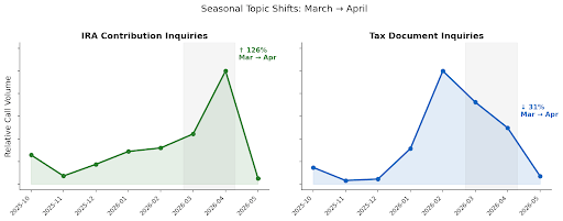
With that, we’ve fully labeled our historical data and can begin extracting useful insights. As an example, we can see how two tax related topics with the same deadline actually have very different call volume profiles over the course of tax season.
Labelling New Data
We have used HDBSCAN so far because it is fast, simple to reason about, and easy to implement. It is also an unsupervised algorithm, so we didn’t need any labelled data to get started. It has a significant drawback though. It can only describe the shape of a closed dataset and cannot be used to label new or held-out data. In order to label newly created call notes, we are going to need something different.
Luckily, we have just created a labelled dataset. While we were previously limited to unsupervised learning models, there are now a plethora of supervised learning models available to us. For our use case, we chose a K-Nearest Neighbors (KNN) model. This post will not cover all the details of training and deploying such a model, but there is plenty of publicly available documentation on using a labelled dataset to train a classifier. Instead, there are a few points to keep in mind about preparing our dataset for training.
Most importantly, this is the best time to clean up our labels. Some labels, especially those created in the third clustering pass, may be so close to each other that it would be better to merge them. An LLM may do a reasonably good job of this, but taking a manual pass over the labels now will be worth the time spent if they will be used for analytical purposes far into the future. Even fully starting over with new clustering parameters is relatively cheap at this point, so we want to be sure we’re happy with our dataset before enshrining it in a classifier.
Another important consideration is how to reencode the data for training. We cannot use the same UMAP approach for dimension reduction the way we did before. When a new datapoint arrives, we need to encode it in the same way as our training data before the model can classify it. UMAP does not allow this. Like HDBSCAN, it is only valid when applied to a closed dataset. One option might be to take a shorter prefix of each embedding returned by the OpenAI model. That is an operation supported by their family of embedding models. We are not, however, constrained to use the same embedding model now as we did to generate our labels. Any model that encodes text to a relatively small number of dimensions will do.
Detecting New Topics
As a final note on using our model to classify new data, we need to address the possibility that new topics will emerge over time. Once we train our classifier, it can assign to a new call any of the topic labels identified in our historical data. But what if the call was about a bug in a product that just launched yesterday? Our model will never be able to immediately identify a new topic like this.
To identify new topics, we need to retrain occasionally. We don’t want to retrain too often because each generation of our model will identify slightly different clusters and we want to preserve stable, long-term labels for downstream analysis. The simplest solution is to pick a regular cadence to retrain. For a more tuned approach, the system can monitor the rate of notes that are not assigned any existing label. When the rate creeps above a fixed threshold, it likely means at least one new cluster has emerged.
We can rerun our original clustering operation over all historical data, including any new data that has arrived since the last time. There will be some unavoidable drift in the existing clusters. Some new data will be grouped into existing clusters from our last iteration, and some existing data may switch clusters. The result is that an existing label like “Withdrawal Inquiries” might have a slightly different meaning than it did before. The LLM naming step might name it slightly differently as well. To mitigate this effect, we can selectively choose to include new data in our training set. Data that was already labelled in a previous iteration can retain its old labels. New data that shares a label with a lot of data that was previously labelled can be omitted. Previously unlabelled data that now shares a label primarily with other previously unlabelled data should definitely be included. Those new labels are the ones we care about most. They capture newly discovered topics.
Disclosures
Investment management and advisory services are provided by Wealthfront Advisers LLC (“Wealthfront Advisers”), an SEC-registered investment adviser, and brokerage related products are provided by Wealthfront Brokerage LLC (“Wealthfront Brokerage”), a Member of FINRA/SIPC. Financial planning tools are provided by Wealthfront Software LLC (“Wealthfront Software”).
The information contained in this communication is provided for general informational purposes only, and should not be construed as investment or tax advice. Nothing in this communication should be construed as a solicitation, offer, or recommendation, to buy or sell any security. Any links provided to other server sites are offered as a matter of convenience and are not intended to imply that Wealthfront Advisers or its affiliates endorses, sponsors, promotes and/or is affiliated with the owners of or participants in those sites, or endorses any information contained on those sites, unless expressly stated otherwise.
Wealthfront Advisers, Wealthfront Brokerage, and Wealthfront Software are wholly-owned subsidiaries of Wealthfront Corporation.
© 2026 Wealthfront Corporation. All rights reserved.