Motivation
You might already know that diversifying your investment over uncorrelated assets is a good way to reduce risk. That’s why people watch asset return correlation closely so they can make informed decision in portfolio construction.
Correlation is important not only in identifying diversification opportunities but also in understanding investment strategies’ characteristics so that we can make informed decision in manager selection.
In this analysis I use return correlation as a similarity measure to cluster some model portfolios listed on Wealthfront platform. I’m hoping that return correlations can reveal these portfolios’ characteristics not easily readable from stated strategies or stock holdings.
Method
I took Wealthfront-listed model portfolios with longer than two-year history, and it resulted a set of 30. For each portfolio, I calculated its monthly returns since inception as a time-series. I then calculated the correlation of monthly returns for each portfolio pairs and constructed a correlation matrix.
I used hierarchical clustering to cluster the portfolios, where the distance measure between each pair of portfolios is given by (1 – return correlation). I chose complete linkage as the linkage function because I want compact and tight clusters of portfolios.
Hierarchical clustering is a clustering method that groups objects into clusters iteratively. It first initializes each object (e.g. portfolio in this analysis) as a cluster. In each iteration, it groups the two closest clusters into a bigger cluster, and gradually builds a cluster tree. The linkage function is used to compute the distance between two clusters. In complete linkage, the distance between two clusters is given by the maximum distance between the objects belonging to each of the two clusters. Complete linkage tends to produce compact and tight clusters.
Note that correlation is the only metric I used to measure and cluster the portfolios. Nothing else.
Results
The portfolio cluster tree constructed by hierarchical clustering is presented in the graph below. Each leaf node is a portfolio, with its ID associated. From bottom up, you can see that hierarchical clustering builds up the cluster tree iteratively by grouping together clusters of portfolios into bigger clusters. The very top level represents the biggest cluster, i.e. the cluster of all 30 portfolios. The height of the tree represents the distance between pairs of clusters, calculated using complete linkage.
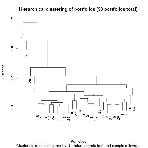
By eye-balling the tree, I would say that the tightest cluster is the one in the left bottom corner. It’s a cluster of nine portfolios, including portfolios 18, 3, 9, 17, 24, 4, 14, 2 and 22. It actually makes a lot of sense, because among them:
– Five portfolios are dividend and growth strategy (portfolio 18, 3, 17, 4 and 14)
– Three portfolios are large-cap strategy (portfolio 9, 24, 22)
– One portfolio is value strategy (portfolio 22)
If you delve into these portfolios’ holdings, you will see that they mostly held/hold large-cap and dividend-paying stocks, and their holdings have a fair amount of overlap. I would categorize this cluster as a large-cap-dividend cluster.
If we draw a horizontal line anchored on the large-cap-dividend cluster sub-tree’s root, you will see another smaller cluster in the middle with similar tightness. It’s the cluster of four including portfolios 11, 12, 13 and 16. Their respective strategies are:
– Portfolios 11 and 12: small+mid-cap strategy
– Portfolio 16: mid-cap strategy
– Portfolio 13: quantitative strategy
The strategy label “quantitative” is vague. It doesn’t say much about the strategy’s essence, nor does it sound related to the other three portfolios. However, if we analyse the portfolio’s holdings, we find that it had and still has a fair portion allocated to mid-cap stocks. The stock holdings of the four portfolios are quite different, but they are all tilted towards the small-cap/mid-cap end of the market-cap spectrum and are relatively highly correlated. I would categorize this cluster as a small+mid-cap cluster.
Another fairly tight cluster is the one with two portfolios, portfolio 19 (strategic asset allocation) and 20 (tactical asset allocation). They both use ETFs to implement asset allocation strategies. No surprise that they ended up in the same cluster.
On the uncorrelated side, portfolio 30 (healthcare), portfolio 28 (value), portfolio 26 (growth) and portfolio 15 (absolute return) are not correlated with the other portfolios (i.e. they are far away from the others on the tree). It makes sense as well because portfolios 30, 28 and 26 are the only portfolios that ever held short positions and thus less correlated with the other long-only portfolios. The most uncorrelated portfolio, i.e. portfolio 15, is absolute return strategy. This portfolio/manager only traded in and out long positions in gold-related instruments, such as gold mutual funds, ETFs and gold miners. That explains its difference from the other stock-focused portfolios.
Discussion
If we only used stated strategies or stock holdings, we wouldn’t have been able to recognize the large-cap-dividend cluster, nor the small+mid-cap cluster identified in this analysis. Nor could we have been able to separate the uncorrelated portfolios into different clusters. Correlation, a statistical measure as basic as it is, through the lens of hierarchical clustering, does offer additional insights into portfolios’ characteristics.
If I were to invest in these portfolios/managers, I’d pick a good manager from the large-cap-dividend cluster, a good manager from the small+mid-cap cluster, and maybe portfolio 15 also (this portfolio is not only uncorrelated with others but also has delivered solid performance consistently). It’s interesting and valuable that return correlation plus hierarchical clustering offer all this practical interpretation for manager selection.